The GW approximation is a workhorse approximation/method in solid state computational materials science, typically used to calculate fairly accurate fundamental gaps of materials. For this blog post, I don’t want to focus on the physics of GW (which is very interesting in itself), but more on the logistical/numerical challenge of extrapolating to the infinite-basis limit for a GW calculation carried out using planewaves as a basis set.

All of the data presented here is from MDB2019, and a particular formula that I’ll be using is inspired from some prose in JK2014.

First we take a look at the leftmost panel in Figure 11 of MDB2019, where we see a few data points of reciprocal of number of planewaves. The authors linearly extrapolate to the infinite basis limit (corresponding to $1/N_G \to 0^+$), where $N_G$ is the number of planewaves used for a particular step of the calculation. However, this involves only taking the last 4 or so points, since for $1/N_G$ larger than that, there are significant deviations from the asymptotically linear trend in $1/N_G$.

Let us quickly motivate what we’re about to do:

1. In JK2014, there are a few lines of prose that go into the higher-order asymptotic terms of the linear expansion in terms of $1/N_G$. The two mentioned there are of the form $1/N_G^{5/3}$ and $1/N_G^{7/3}$. For a simple exploration like the one here, we can just stick to the effects of the first higher-order term.
2. In MDB2019, the linear asymptotic trend really only sets in for higher planewave counts. We want to improve on this situation, since GW calculations rapidly get more expensive as a function of the number of planewaves. It therefore behooves us to find an extrapolation method that performs accurately without high-planewave-count calculations. We desire not just to extrapolate, but to extrapolate quickly.

First, we need to extract the data from Fig 11 in MDB2019. We use WebPlotDigitizer for this. The final data table for energy vs $1/N_G$ comes out to (this can change slightly depending on every extraction, the actual numbers are not really important beyond ~2-3 sigfigs):

0.0001823736780258519, 2.6465870307167236
0.00021245593419506455, 2.6436860068259387
0.00025569917743830783, 2.6392491467576793
0.00031774383078730884, 2.6331058020477816
0.0003948296122209166, 2.6237201365187715
0.0005236192714453587, 2.608873720136519
0.0007210340775558165, 2.58259385665529

where the first column is the reciprocal number of planewaves, and the second number is the calculated band gap at that basis set size.

We can write the above data to a file, call it (among an infinite number of possible names) datafile.csv, and we can then read in the data as below. Note the rescaling, which doesn’t affect any of our results that we will care about, and is generally good practice when fitting (the $1/N_G$ numbers are much smaller than ~1, so we rescale to something nicer).

import numpy as np

data = np.loadtxt('datafile.csv', delimiter=',')
data[:, 0] /= np.max(data[:, 0]) # Rescale 1/N_Gs closer to 1

Linear extrapolation, part 1

We will now extrapolate via linear extrapolation to the infinite-planewaves limit:

# This code needs to be pasted after the last line of the previous code block

linearfit_fulldata_coeffs = []
# Let's also find out how well the extrapolation works as we
# use lower-pw-count data points by omitting high-pw-count
# data points one by one.
for i in range(4):
    coeff = np.polyfit(data[i:, 0], data[i:, 1], deg=1)
    linearfit_fulldata_coeffs.append(coeff[-1])
    print(coeff)

The above piece of code should print out either exactly, or something similar to:

[-0.08543527  2.66954407]
[-0.0866261   2.67043627]
[-0.08811155  2.67159317]
[-0.0900937   2.67321259]

where the second number in each line is the y-intercept of the linear fit. This is the number we care about, since this is the band gap at $1/N_G \to 0^+$. It’s not moving a lot, but can we do better?

Linear extrapolation, part 2

Before we answer that, a quick aside. In the above snippet, we used the entire dataset, including points which we can see are obviously not linear. What happens if we omit the last 2 points in the dataset, for which the deviation from linear is the highest:

linearfit_lineardata_coeffs = []
# Let's also find out how well the extrapolation works as we
# use lower-pw-count data points by omitting high-pw-count
# data points one by one.
for i in range(2):
    coeff = np.polyfit(data[i:-2, 0], data[i:-2, 1], deg=1)
    linearfit_lineardata_coeffs.append(coeff[-1])
    print(coeff)

which gives us exactly, or something similar to:

[-0.07712152  2.666429  ]
[-0.07856926  2.66710552]

Higher-order extrapolation

Coming back to the question of can we do better, we now define a custom fit function that will take into account higher-order asymptotic behaviour:

def gap_asymptotic(recip_ng, a, b, c):
    return a * recip_ng + b * recip_ng ** (5/3) + c

where we’ve taken into account the first higher-order term.

We can then proceed as above, replacing the polyfit with our custom fit function and Scipy’s curve_fit:

from scipy.optimize import curve_fit
hofit_coeffs = [] # ho for higher-order
for i in range(4):
    coeff, cov = curve_fit(gap_asymptotic, data[i:, 0], data[i:, 1])
    hofit_coeffs.append(coeff[-1])
    print(coeff)

which should print out something similar to:

[-0.04820859 -0.0311096   2.66194399]
[-0.04842447 -0.03094642  2.66199929]
[-0.04858706 -0.03082633  2.6620432 ]
[-0.05279223 -0.02780813  2.66325221]

where the third number in each array is the band gap at $1/N_G \to 0^+$. We see that this number now moves a lot less as we reduce the number of points for the fit!

More importantly: The largest planewave-count calculation is now much smaller compared to the first two linear extrapolation attempts. Since we are taking into account higher-order asymptotic terms, the asymptotic behaviour can be sufficiently accurately described for much larger $1/N_G$ (equivalently, much smaller number of planewaves).

Now let us plot out the result of the extrapolation procedure as a gap vs points-omitted-from-extrapolation plot

import matplotlib.pyplot as plt
x = np.arange(0, 4)
plt.figure(figsize=(5, 4), dpi=150, facecolor='white')
plt.plot(x, linearfit_fulldata_coeffs, '.-', label='Linear, all data')
plt.plot(x[:-2], linearfit_lineardata_coeffs, 'x-', label='Linear, picked data')
plt.plot(x, hofit_coeffs, 'o-', label='Higher-order, all data')
plt.xticks(x, labels=x)
plt.legend(frameon=False)
plt.ylabel('Extrapolated gap [eV]')
plt.xlabel('Omitted GW calculations')
plt.tight_layout()
plt.show()

which gives us:

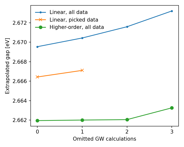
We see how the band gap converges much earlier to a tolerance that iscomparable to both linear extrapolations. More importantly, we can omit up to 4 of the above most expensive GW calculations (with the highest planewave counts) and still get a very converged value for the band gap (which is already ~2 orders of magnitude more accurate than the intrinsic error of the GW method compared to experiment). The fact that all three extrapolations yield different final answers can be quantified with fit uncertainties. But the effort is likely not worth it (unless to prove a point) since the error between GW and experimental values is already ~0.1-0.2 eV typically, orders of magnitude higher than the extrapolation error.

Conclusions:

1. We can save huge amounts of computational resources by doing GW calculations with smaller planewave counts if we extrapolate using higher-order asymptotic expressions for the extrapolated quantity (here, the band gap).
2. Using high-order asymptotics removes the need to hand-pick data points which have linear behaviour (although this can probably be taken care of robust linear regression).

Full code:

import numpy as np

data = np.loadtxt('datafile.csv', delimiter=',')
data[:, 0] /= np.max(data[:, 0]) # Rescale 1/N_Gs closer to 1
# This code needs to be pasted after the last line of the previous code block

linearfit_fulldata_coeffs = []
# Let's also find out how well the extrapolation works as we
# use lower-pw-count data points by omitting high-pw-count
# data points one by one.
for i in range(4):
    coeff = np.polyfit(data[i:, 0], data[i:, 1], deg=1)
    linearfit_fulldata_coeffs.append(coeff[-1])
    print(coeff)

linearfit_lineardata_coeffs = []
# Let's also find out how well the extrapolation works as we
# use lower-pw-count data points by omitting high-pw-count
# data points one by one.
for i in range(2):
    coeff = np.polyfit(data[i:-2, 0], data[i:-2, 1], deg=1)
    linearfit_lineardata_coeffs.append(coeff[-1])
    print(coeff)

def gap_asymptotic(recip_ng, a, b, c):
    return a * recip_ng + b * recip_ng ** (5/3) + c

from scipy.optimize import curve_fit
hofit_coeffs = [] # ho for higher-order
for i in range(4):
    coeff, cov = curve_fit(gap_asymptotic, data[i:, 0], data[i:, 1])
    hofit_coeffs.append(coeff[-1])
    print(coeff)

import matplotlib.pyplot as plt
x = np.arange(0, 4)
plt.figure(figsize=(5, 4), dpi=150, facecolor='white')
plt.plot(x, linearfit_fulldata_coeffs, '.-', label='Linear, all data')
plt.plot(x[:-2], linearfit_lineardata_coeffs, 'x-', label='Linear, picked data')
plt.plot(x, hofit_coeffs, 'o-', label='Higher-order, all data')
plt.xticks(x, labels=x)
plt.legend(frameon=False)
plt.ylabel('Extrapolated gap [eV]')
plt.xlabel('Omitted GW calculations')
plt.tight_layout()
plt.show()

EDIT 1 (15-May-2022): The work referenced by JK2014 which is listed as unpublished in their bibliography (at least in the version of the paper I have access to) has been included in the references AG2014 since there are a few nice plots there for extrapolation including higher-order terms (figures 1, 2, 3). It also has a full exposition of the physics that leads to the asymptotic expansion, although this is much more involved than just a quick fun blog post on extrapolation effects.

References:

MDB2019

JK2014

AG2014