How much data do we need to stabilize an MLIP?

Machine learned interatomic potentials have become are now frontline tools in materials science, and are used for a variety of statistical (and otherwise) sampling tasks. However, unlike a potential with a closed form expression for energies/forces/stresses, MLIPs do not usually have a repulsive core potential when two atoms approach each other.

Exceptions like MACE-MPA-0 exist, with a robust core repulsion. As does 7net, the Orb potentials, a few others, see the MLIPX page. But in general, you will eventually run into some form of nuclear fusion. Somewhere, a C-C bond will become 0.3 angstrom, a B-N bond will become 0.4 angstrom, and so on.

But even with fixes/near-fixes for the ‘nuclear fusion problem’, it’s a problem worth exploring how to mitigate. MACE-MPA-0 is (compared to some other MLIP architectures) quite slow. This is not beating on MACEp; most foundation potentials are quite hefty and have time/atom-step limitations (unless they’ve been blessed by the NVIDIA engineers).

Cue Apax. This is an implementation of the GMNN MLIP architecture developed by Moritz Schaefer. It’s quite fast (I trained the models on here on a CPU on WSL…), I invite you to find out just how fast. I’m pretty sure it goes sub-microsecond/atom on an H100 or a high-end Blackwell card. It’s also extremely light on memory use, no message-passing beyond the first radial basis (as of this writing, although we’ve toyed with the idea), and so on. Unfortunately, it’s also quite finicky (or at least as been) in terms of stability. The unconstrained neural net ‘backend’ is at least somewhat unstable in the close-approach region.

For comparison, MACE/ACE does an Agnesi transform of the radial coordinate and suppresses the close-approach output from non-2-body terms see here. The UPET models are trained on a dataset that contains close-approach dimers. This is a perfectly valid suggestion, but of course I, as a spoiled scientist, just want a problem to Go Away.

Apax has a ZBL repulsion empirical correction option, but we’ll see the limitations with it. Let’s build a potential without it and see what we get. We’re going to use an ethanol dataset that’s just a single molecule of ethanol wiggling about.

To test the potential outside the range where it has data, (but where we still like it to be at least qualitatively correct), we will use a comprehesive closest approach test. We will create a neighborlist with a 1.6 angstrom cutoff (just above C-C single bonds), then, for each unique bond, we will make one atom approach the other along the bond vector from whatever the equilibrium length is, to 0.1 angstrom. I consider this to be a much more comprehensive test than a homonuclear dimer approach, or any sort of dimer-approach test. We are trying to make sure that regardless of the local environment, two atoms approaching each other leads to energies blowing up (smoothly and monotonically).

Here’s the code. Claude wrote it, I checked it. Not even I am immune to outsourcing tedium. The first one generates the approach scans, the second one uses a trained Apax model to plot the energies given the scan trajectories.

import numpy as np
from ase.io import read, write
from ase.neighborlist import neighbor_list

FINAL = 0.1   # Ang
NSTEPS = 20

atoms = read("etoh.traj", index=0)

sym = atoms.get_chemical_symbols()
i, j = neighbor_list("ij", atoms, 1.6)
pairs = {(a, b) for a, b in zip(i, j) if a < b}  # unique

for a, b in sorted(pairs):
    pair_type = {sym[a], sym[b]}
    stretch = pair_type in ({"C", "H"}, {"O", "H"})  # X-H: stretch, move only H
    frames = []
    for s in range(NSTEPS):
        img = atoms.copy()
        p = img.positions
        d = img.get_distance(a, b)
        if stretch:
            h, x = (a, b) if sym[a] == "H" else (b, a)
            target = 2 * d + (FINAL - 2 * d) * s / (NSTEPS - 1)  # linear 2d -> 0.1
            u = (p[h] - p[x]) / d
            p[h] = p[x] + u * target  # keep heavy atom fixed
        else:
            mid = (p[a] + p[b]) / 2
            target = d + (FINAL - d) * s / (NSTEPS - 1)  # linear d -> 0.1
            u = (p[b] - p[a]) / d
            p[a] = mid - u * target / 2
            p[b] = mid + u * target / 2
        frames.append(img)
    write(f"approach_{a}_{b}.traj", frames)

print(f"{len(pairs)} pairs written")

import glob
import sys
import matplotlib.pyplot as plt
from ase.io import read
from apax.md import ASECalculator

model = sys.argv[1] if len(sys.argv) > 1 else "models/apax"
calc = ASECalculator(model)

for f in sorted(glob.glob("approach_*.traj")):
    a, b = (int(x) for x in f[:-5].split("_")[1:])
    frames = calc.batch_eval(read(f, ":"))
    sym = frames[0].get_chemical_symbols()
    d = [img.get_distance(a, b) for img in frames]
    e = [img.get_potential_energy() for img in frames]
    plt.plot(d, e, "o-", label=f"{sym[a]}{a}-{sym[b]}{b}")

plt.ylim(-4220, -4200)
plt.xlabel("distance (Ang)")
plt.ylabel("energy (eV)")
plt.legend()
plt.tight_layout()
out = f"approach_energies_{model.split('/')[-1]}.png"
plt.savefig(out, dpi=150)
print("wrote", out)

What happens?

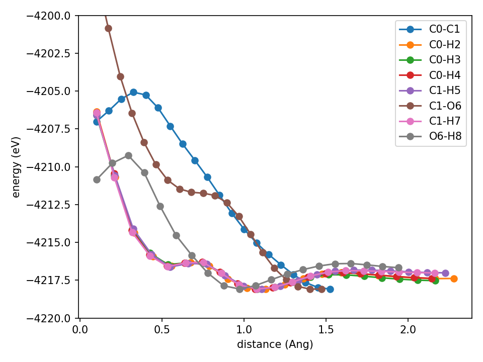
Tragedy has struck quite immediately. The approach energy curves are not monotonic, they don’t diverge to +infinity at 0, turn downwards near 0, all of the things we would like to not have, regardless of the quantitative correctness of the trained potential.

At some level, this is not unexpected. So we turn on repulsion and retrain. We train once with 16 basis functions, but then (a bit of cheating here, I’ve seen this phenomenon before, so I know that remotely touching any model parameter can cause it) I retrain with 8 and 24 basis functions and there we go. The close-approach regions look quite not great. This is even with a ZBL repulsion term. We have no verified that the problem exists.

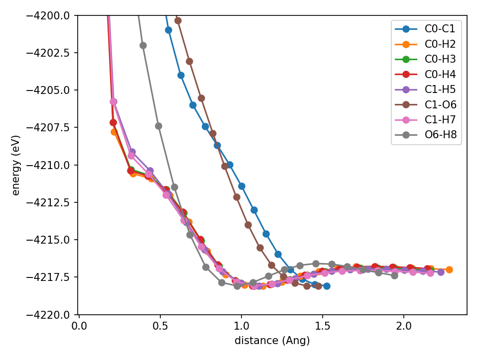
What about when we add the standard ZBL that Apax has?

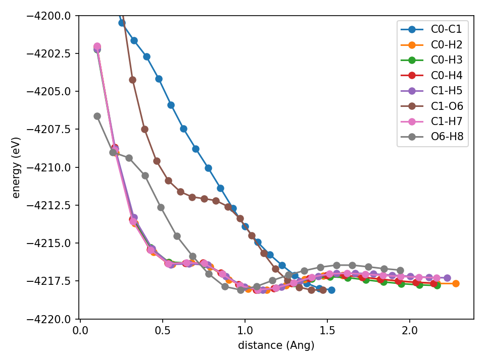
Slightly better but it’s really not good. The O6-H8 curve is better, but C1-H7 has a spurious minimum at ~0.6 angstrom. You may think this isn’t all that bad. But I’ve see much worse (it depends a bit randomly on initialization, seed, etc). So I reduce the basis function count to 8 (just any change to get something interesting to happen).

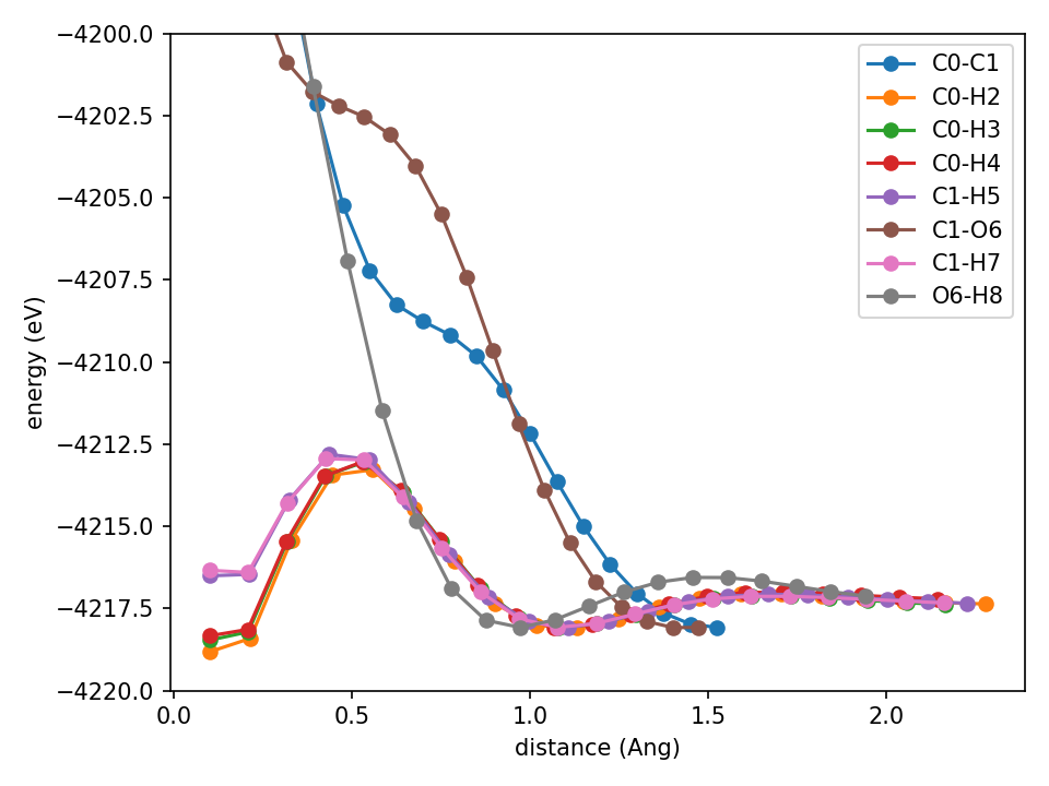
This is bad. All of the hydrogen-containing curves are now garbage. What about 24 basis functions?

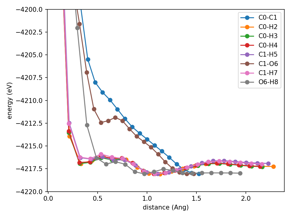
Spurious minima, all the bads.

What changes do we make to “fix” this?

I put fix in quotes since it’s not a rigorous fix that is mathematically provable to always be correct. This is more of an empirical fix that we hope will work the overwhelming majority of the time.

The first thing that comes to mind from a stereotypical physicist perspective (at least to me) is ‘bound the hamiltonian from below’. What this means is that instead of the readout being a linear readout, add a bounded activation for the atomistic readout module in apax. This is then fed into the scale-shift, so if we bound the readout from below, we’ve got a bounded hamiltonian. This by itself doesn’t solve the repulsion issue, but it does prevent unbounded negative values from the NN in data-poor regions.

So we implement it, and because this is more of a leisurely activity and not rigorous experimentation, I also ramp up the empirical ZBL repulsion’s ‘repulsion scale’, which is essentially a trainable fudge-prefactor. It was initialized at 0.1 for the above runs, I initialize it to 1.0. I’ve sometimes had bad luck in terms of training stability with this, but I’ll try to systematically reproduce that and talk about it at a later date.

Finally some good monotonic repulsion.

I don’t have a big paragraph of conclusion. Here’s a bulleted list of things that I believe have helped.

1. Bounding the ‘Hamiltonian’ (NN) from below using a swish activation function.
2. Increasing the strength of the ZBL repulsion at initialization, the rest of the NN updates quickly before the repulsion is killed/the prefactor is trained away.